From Backtest to Production: a Bot Architecture Path

A strategy that looks great in a notebook and loses money live usually did not get worse — it got measured differently. The backtest ran on cleaned candles while production sees raw ticks; the backtest filled instantly at mid while production queues at the touch; the backtest's clock was the candle close while production's is a feed with jitter. This guide describes the architecture path we recommend to close those gaps one stage at a time — using self-serve pieces where possible.

The four stages

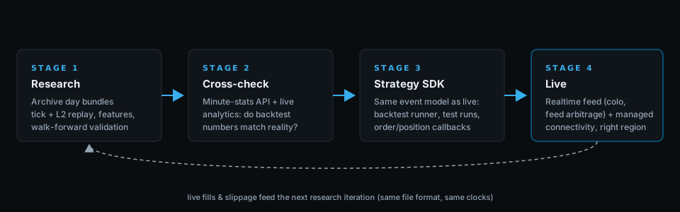
Stage 1 — research on the archive, at tick resolution

Start where iteration is cheapest: historical files. Archive days cost €1 per instrument-day (or per series-day bundle on prediction venues) and contain the full L2 order-book path plus every trade at nanosecond timestamps — enough to build queue-aware fill models and charge real spread-crossing costs instead of assuming mid-price fills. (L2 data cannot tell you your exact place in the queue; it lets you estimate it with an explicit queue model rather than ignore it.) Parse with the free Python reader or the one-click CSV/Parquet exports, and validate walk-forward (the training-data guide covers splits and label hygiene).

Stage 2 — cross-check against an independent implementation

Before trusting your parser and aggregation code, reconcile them against numbers you did not compute. The free per-minute statistics API serves OHLC, VWAP, trade counts, turnover, spreads and book depth per minute for every instrument — computed by an independent implementation from the same recordings. The comparison validates your parser and aggregation path, not the original exchange capture, which both sides share. Aggregate your tick-level results to minutes and diff them: a persistent mismatch usually indicates a parsing, normalization or aggregation difference that should be investigated (aggressor-side mix-ups and quote-currency confusion are the classics). The live analytics give the same numbers visually for spot checks.

Stage 3 — port into an event model that also runs live

The subtle production killer is the programming model: research code is usually vectorized over a whole day, while live code reacts to one event at a time. Port your strategy into an event-driven harness before going live — ours is the Strategy SDK (Java): you implement callbacks for book changes, trades, order updates and timers, and the same class runs in the backtest runner and in production. The tutorial series walks from first strategy to local backtesting. Whatever SDK you use, the invariant to enforce is: one strategy artifact, two runners — never two implementations.

Stage 4 — shadow, then go live on the feed the archive came from

In production, data quality becomes latency-shaped: you care about jitter, gaps and tails. The archive you researched on was recorded from our co-located realtime feeds — going live on those feeds keeps capture and normalization identical between research and production, which removes one major source of train/live distribution shift (normalized schema, exchange timestamps, feed arbitrage against jitter; from €1,000 per API and month with a two-week free test, and the first 30 days of history included as an initial dump). Deployment placement — regions, links, how to measure your own feed delay — has its own guide: Where to run your prediction-market bot. For dedicated lines, RF routes and co-located hardware, talk to us.

Ramp up, don't switch on

1. Shadow mode: run the strategy on the live feed with orders logged, not sent — and diff its decisions and hypothetical fills against the backtest runner on the same days.
2. Canary size: send real orders at minimum size; measure fill ratio, slippage, reject rate and feed delay against your backtest assumptions.
3. Scale up only when the live metrics sit inside the tolerance you set in research — and keep the shadow comparison running as a regression check.

Production risks the backtest never sees

An event-driven port and a careful ramp-up still leave a class of failure modes no historical file contains — the live order path itself. Budget engineering time for at least these before scaling up:

• Order latency and rejects — the venue can answer slowly, or with an error; every reject path needs a tested handler.
• Rate limits — order, cancel and data requests are throttled per venue; bursts that were free in the backtest can lock you out live.
• Disconnects and reconnects — sessions drop; resyncing the book and your open-order state after a gap must be automatic.
• Stale or degraded feeds — detect when data stops being trustworthy and stop quoting instead of trading on it.
• Order-state reconciliation — periodically confirm positions and open orders against the venue; local state drifts after any hiccup.
• Callback and event ordering — live events can interleave in ways the backtest never produced; strategy logic must not depend on a fortunate ordering.

This is why the loop below starts with recording your live fills, quotes and rejects — those logs are also your incident forensics. The trading API documentation covers the live order path in detail.

Close the loop

1. Record your live fills, quotes and rejects with the same timestamp discipline as the market data.
2. Rebuild your backtest's fill model from measured live slippage — not the other way around.
3. Re-run the research pipeline on fresh archive days every few weeks; models drift with regimes.
4. Alert on distribution shifts between backtest assumptions and live measurements (spread, fill ratio, feed delay p99).
5. Keep one metric dashboard for both runners — if backtest and live are not comparable at a glance, the loop is open.

Limitations

This is an architecture guide, not a strategy recipe: following it makes results measurable and transferable, not profitable. Pricing facts (€1 archive days, realtime terms) are current as of August 2026 — the pricing page is authoritative. The SDK examples reference our Java stack; the staging logic applies to any event-driven framework. Nothing here is investment advice.